import numpy as np
import pandas as pd

import matplotlib.pyplot as plt
import seaborn as sns

import tensorflow as tf
from sklearn.datasets import fetch_california_housing

ds = fetch_california_housing()
ds.DESCR
'.. _california_housing_dataset:\n\nCalifornia Housing dataset\n--------------------------\n\n**Data Set Characteristics:**\n\n:Number of Instances: 20640\n\n:Number of Attributes: 8 numeric, predictive attributes and the target\n\n:Attribute Information:\n - MedInc median income in block group\n - HouseAge median house age in block group\n - AveRooms average number of rooms per household\n - AveBedrms average number of bedrooms per household\n - Population block group population\n - AveOccup average number of household members\n - Latitude block group latitude\n - Longitude block group longitude\n\n:Missing Attribute Values: None\n\nThis dataset was obtained from the StatLib repository.\nhttps://www.dcc.fc.up.pt/~ltorgo/Regression/cal_housing.html\n\nThe target variable is the median house value for California districts,\nexpressed in hundreds of thousands of dollars ($100,000).\n\nThis dataset was derived from the 1990 U.S. census, using one row per census\nblock group. A block group is the smallest geographical unit for which the U.S.\nCensus Bureau publishes sample data (a block group typically has a population\nof 600 to 3,000 people).\n\nA household is a group of people residing within a home. Since the average\nnumber of rooms and bedrooms in this dataset are provided per household, these\ncolumns may take surprisingly large values for block groups with few households\nand many empty houses, such as vacation resorts.\n\nIt can be downloaded/loaded using the\n:func:`sklearn.datasets.fetch_california_housing` function.\n\n.. rubric:: References\n\n- Pace, R. Kelley and Ronald Barry, Sparse Spatial Autoregressions,\n Statistics and Probability Letters, 33 (1997) 291-297\n'
X = ds.data
y = ds.target
X.shape
(20640, 8)
y.shape
(20640,)
from sklearn.model_selection import train_test_split

X_train, X_test, y_train, y_test = train_test_split(X, y, test_size=0.3, random_state=101)
from sklearn.preprocessing import StandardScaler

scaler = StandardScaler()
scaler.fit(X_train)

X_train = scaler.transform(X_train)
X_test = scaler.transform(X_test)
from tensorflow.keras.models import Sequential
#help(Sequential)
from tensorflow.keras.layers import Input, Dense, Activation
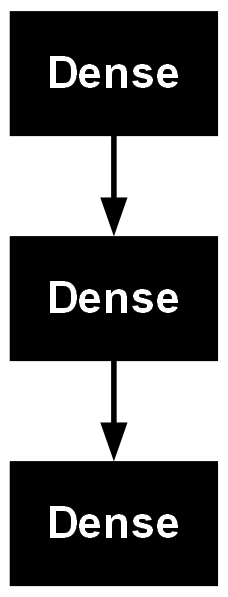
model = Sequential()
model.add(Input(shape=(8,))) # 8 features, so 8 inputs
model.add(Dense(8, activation='relu')) # first layer
model.add(Dense(4, activation='relu')) # hidden layer
model.add(Dense(1)) # output layer, 1 output (predicted value)
model.compile(optimizer='adam', loss='mse')
model.summary()
Model: "sequential"
┏━━━━━━━━━━━━━━━━━━━━━━━━━━━━━━━━━━━━━━┳━━━━━━━━━━━━━━━━━━━━━━━━━━━━━┳━━━━━━━━━━━━━━━━━┓
┃ Layer (type)                         ┃ Output Shape                ┃         Param # ┃
┡━━━━━━━━━━━━━━━━━━━━━━━━━━━━━━━━━━━━━━╇━━━━━━━━━━━━━━━━━━━━━━━━━━━━━╇━━━━━━━━━━━━━━━━━┩
│ dense (Dense)                        │ (None, 8)                   │              72 │
├──────────────────────────────────────┼─────────────────────────────┼─────────────────┤
│ dense_1 (Dense)                      │ (None, 4)                   │              36 │
├──────────────────────────────────────┼─────────────────────────────┼─────────────────┤
│ dense_2 (Dense)                      │ (None, 1)                   │               5 │
└──────────────────────────────────────┴─────────────────────────────┴─────────────────┘
Total params: 113 (452.00 B)
Trainable params: 113 (452.00 B)
Non-trainable params: 0 (0.00 B)
model.fit(X_train, y_train, epochs=50, verbose=1)
Epoch 1/50
452/452 ━━━━━━━━━━━━━━━━━━━━ 1s 606us/step - loss: 2.8958
Epoch 2/50
452/452 ━━━━━━━━━━━━━━━━━━━━ 0s 607us/step - loss: 0.7722
Epoch 3/50
452/452 ━━━━━━━━━━━━━━━━━━━━ 0s 608us/step - loss: 0.5616
Epoch 4/50
452/452 ━━━━━━━━━━━━━━━━━━━━ 0s 600us/step - loss: 0.5029
Epoch 5/50
452/452 ━━━━━━━━━━━━━━━━━━━━ 0s 604us/step - loss: 0.4529
Epoch 6/50
452/452 ━━━━━━━━━━━━━━━━━━━━ 0s 592us/step - loss: 0.4192
Epoch 7/50
452/452 ━━━━━━━━━━━━━━━━━━━━ 0s 602us/step - loss: 0.4210
Epoch 8/50
452/452 ━━━━━━━━━━━━━━━━━━━━ 0s 584us/step - loss: 0.3912
Epoch 9/50
452/452 ━━━━━━━━━━━━━━━━━━━━ 0s 585us/step - loss: 0.3792
Epoch 10/50
452/452 ━━━━━━━━━━━━━━━━━━━━ 0s 581us/step - loss: 0.3750
Epoch 11/50
452/452 ━━━━━━━━━━━━━━━━━━━━ 0s 611us/step - loss: 0.3801
Epoch 12/50
452/452 ━━━━━━━━━━━━━━━━━━━━ 0s 642us/step - loss: 0.3714
Epoch 13/50
452/452 ━━━━━━━━━━━━━━━━━━━━ 0s 589us/step - loss: 0.3631
Epoch 14/50
452/452 ━━━━━━━━━━━━━━━━━━━━ 0s 587us/step - loss: 0.3453
Epoch 15/50
452/452 ━━━━━━━━━━━━━━━━━━━━ 0s 598us/step - loss: 0.3537
Epoch 16/50
452/452 ━━━━━━━━━━━━━━━━━━━━ 0s 599us/step - loss: 0.3459
Epoch 17/50
452/452 ━━━━━━━━━━━━━━━━━━━━ 0s 595us/step - loss: 0.3491
Epoch 18/50
452/452 ━━━━━━━━━━━━━━━━━━━━ 0s 584us/step - loss: 0.3321
Epoch 19/50
452/452 ━━━━━━━━━━━━━━━━━━━━ 0s 650us/step - loss: 0.3349
Epoch 20/50
452/452 ━━━━━━━━━━━━━━━━━━━━ 0s 633us/step - loss: 0.3508
Epoch 21/50
452/452 ━━━━━━━━━━━━━━━━━━━━ 0s 634us/step - loss: 0.3499
Epoch 22/50
452/452 ━━━━━━━━━━━━━━━━━━━━ 0s 625us/step - loss: 0.3365
Epoch 23/50
452/452 ━━━━━━━━━━━━━━━━━━━━ 0s 640us/step - loss: 0.3421
Epoch 24/50
452/452 ━━━━━━━━━━━━━━━━━━━━ 0s 653us/step - loss: 0.3274
Epoch 25/50
452/452 ━━━━━━━━━━━━━━━━━━━━ 0s 638us/step - loss: 0.3300
Epoch 26/50
452/452 ━━━━━━━━━━━━━━━━━━━━ 0s 678us/step - loss: 0.3288
Epoch 27/50
452/452 ━━━━━━━━━━━━━━━━━━━━ 0s 640us/step - loss: 0.3317
Epoch 28/50
452/452 ━━━━━━━━━━━━━━━━━━━━ 0s 596us/step - loss: 0.3266
Epoch 29/50
452/452 ━━━━━━━━━━━━━━━━━━━━ 0s 596us/step - loss: 0.3227
Epoch 30/50
452/452 ━━━━━━━━━━━━━━━━━━━━ 0s 591us/step - loss: 0.3133
Epoch 31/50
452/452 ━━━━━━━━━━━━━━━━━━━━ 0s 615us/step - loss: 0.3124
Epoch 32/50
452/452 ━━━━━━━━━━━━━━━━━━━━ 0s 683us/step - loss: 0.3253
Epoch 33/50
452/452 ━━━━━━━━━━━━━━━━━━━━ 0s 608us/step - loss: 0.3349
Epoch 34/50
452/452 ━━━━━━━━━━━━━━━━━━━━ 0s 595us/step - loss: 0.3197
Epoch 35/50
452/452 ━━━━━━━━━━━━━━━━━━━━ 0s 681us/step - loss: 0.3120
Epoch 36/50
452/452 ━━━━━━━━━━━━━━━━━━━━ 0s 647us/step - loss: 0.3105
Epoch 37/50
452/452 ━━━━━━━━━━━━━━━━━━━━ 0s 792us/step - loss: 0.3242
Epoch 38/50
452/452 ━━━━━━━━━━━━━━━━━━━━ 0s 661us/step - loss: 0.3095
Epoch 39/50
452/452 ━━━━━━━━━━━━━━━━━━━━ 0s 659us/step - loss: 0.3096
Epoch 40/50
452/452 ━━━━━━━━━━━━━━━━━━━━ 0s 646us/step - loss: 0.3124
Epoch 41/50
452/452 ━━━━━━━━━━━━━━━━━━━━ 0s 768us/step - loss: 0.3161
Epoch 42/50
452/452 ━━━━━━━━━━━━━━━━━━━━ 0s 650us/step - loss: 0.3085
Epoch 43/50
452/452 ━━━━━━━━━━━━━━━━━━━━ 0s 663us/step - loss: 0.3156
Epoch 44/50
452/452 ━━━━━━━━━━━━━━━━━━━━ 0s 665us/step - loss: 0.3057
Epoch 45/50
452/452 ━━━━━━━━━━━━━━━━━━━━ 0s 622us/step - loss: 0.3133
Epoch 46/50
452/452 ━━━━━━━━━━━━━━━━━━━━ 0s 649us/step - loss: 0.3103
Epoch 47/50
452/452 ━━━━━━━━━━━━━━━━━━━━ 0s 694us/step - loss: 0.3148
Epoch 48/50
452/452 ━━━━━━━━━━━━━━━━━━━━ 0s 831us/step - loss: 0.3077
Epoch 49/50
452/452 ━━━━━━━━━━━━━━━━━━━━ 0s 695us/step - loss: 0.3048
Epoch 50/50
452/452 ━━━━━━━━━━━━━━━━━━━━ 0s 680us/step - loss: 0.3033
<keras.src.callbacks.history.History at 0x243da1064b0>
from tensorflow.keras.utils import plot_model
plot_model(model)
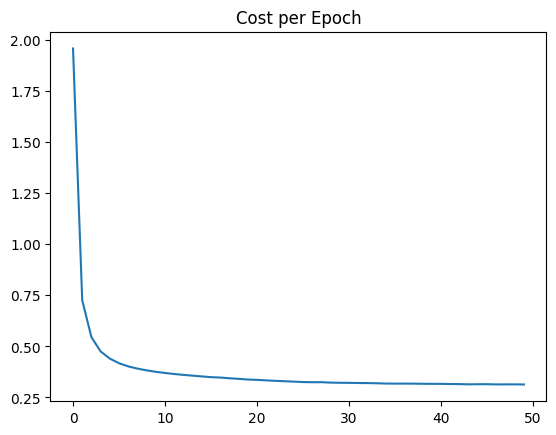
loss = model.history.history['loss']
sns.lineplot(x=range(len(loss)), y=loss)
plt.title("Cost per Epoch");
model.evaluate(X_test, y_test, verbose=0) # gives MSE on test data
0.3631080389022827
predictions = model.predict(X_test)
194/194 ━━━━━━━━━━━━━━━━━━━━ 0s 661us/step
predictions_df = pd.DataFrame(y_test, columns=['Actual value'])
predictions = pd.Series(predictions.reshape(predictions.shape[0],))
predictions_df = pd.concat([predictions_df, predictions], axis=1)
predictions_df.columns = ['Actual value', 'Prediction']
predictions_df['Error'] = predictions_df['Prediction'] - predictions_df['Actual value']
predictions_df['AbsError'] = predictions_df['Error'].abs()
predictions_df.head()
| Actual value | Prediction | Error | AbsError | |
|---|---|---|---|---|
| 0 | 4.06200 | 3.373669 | -0.688331 | 0.688331 |
| 1 | 5.00001 | 5.458389 | 0.458379 | 0.458379 |
| 2 | 1.22900 | 1.307656 | 0.078656 | 0.078656 |
| 3 | 2.09100 | 1.761254 | -0.329746 | 0.329746 |
| 4 | 5.00001 | 4.051704 | -0.948306 | 0.948306 |
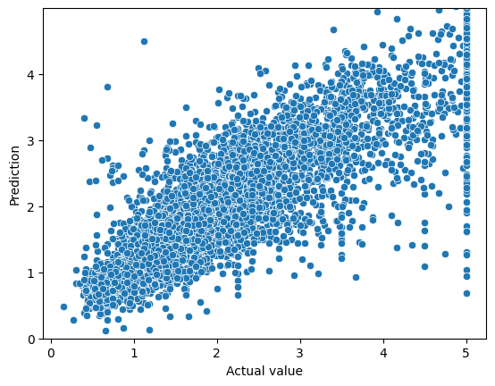
fig, ax = plt.subplots()
sns.scatterplot(x='Actual value', y='Prediction', data=predictions_df, ax=ax)
ax.set_ylim(0,5)
ax.set_yticks(range(0,5))
[<matplotlib.axis.YTick at 0x243dff3d400>,
 <matplotlib.axis.YTick at 0x243dcce1c70>,
 <matplotlib.axis.YTick at 0x243dff3f980>,
 <matplotlib.axis.YTick at 0x243dffc0d70>,
 <matplotlib.axis.YTick at 0x243dff4f560>]
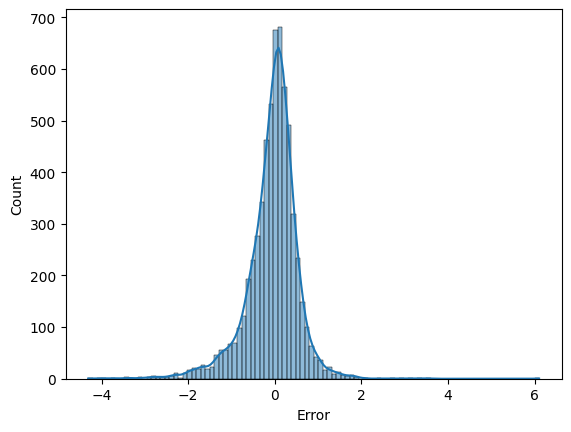
sns.histplot(predictions_df['Error'], bins=100, kde=True)
<Axes: xlabel='Error', ylabel='Count'>
from sklearn.metrics import mean_squared_error
mean_squared_error(predictions_df['Actual value'], predictions_df['Prediction']) # should match MSE given by model.evaluate()
0.36310797841447406
predictions_df['AbsError'].mean()
0.41034741368234623
from sklearn.metrics import mean_absolute_error
mean_absolute_error(predictions_df['Actual value'], predictions_df['Prediction']) # should match MAE in cell above
0.41034741368234623
model.layers
[<Dense name=dense, built=True>,
 <Dense name=dense_1, built=True>,
 <Dense name=dense_2, built=True>]
# get the hidden layer and get its weights and biases
hidden1 = model.layers[1]
weigths,biases = hidden1.get_weights()
weigths
array([[-1.5367666 ,  0.5578632 ,  0.91849107,  0.4004497 ],
       [ 0.48640004,  0.30859554,  1.2143872 ,  0.51258546],
       [-1.1379403 ,  0.34243038, -0.50819266, -0.25250834],
       [-0.17888296,  0.26494405, -0.89329773, -0.2557593 ],
       [-0.48211303, -0.10195341,  0.38939202, -0.40084916],
       [ 0.5273591 , -0.07975588, -0.4525347 ,  0.5942349 ],
       [ 0.32114583, -1.2568455 , -1.1789087 , -1.1678939 ],
       [-0.59614944,  0.61493313, -0.56319606,  0.09937736]],
      dtype=float32)
biases
array([0.5820168 , 0.20370772, 0.00558734, 0.46961448], dtype=float32)